Demography now
Kimmo Klemola
23.05.2006
Demography deals with populations. It is much more important than democracy.
In 1908, German chemist Fritz Haber made an innovation that probably outplays all other innovations of the 20th century. He succeeded in combining fossil energy in a form of hydrogen steam reformed from natural gas into nitrogen distilled from the air to obtain ammonia. Ammonia is a raw material in the production of nitric acid that is further manufactured to fertilizers and explosives. Industrial fertilizers enabled industrial agriculture and were the prime reason for population explosion. Without Haber's innovation there would be maybe only half of the current population on earth. World population is growing at a rate of 200,000 a day or 74 million a year – twice the population of Poland.
Population projections are estimates of the population for future dates. Population projection math is based on numerical solutions of differential equation systems. Here I present a simple world population projection and a more detailed projection for US population. Initial population data and certain parameters such as birth rates, death rates and net immigration rates are needed. Numerical mathematics programs such as Matlab or Polymath can easily do the numerical integration of the differential equation system.
The difficulty is in determining reliable parameters that may be inherently time dependent and very uncertain. Pandemics such as AIDS, global starvation, peak oil, economic crises etc. can strongly affect birth and death rates and local net immigration rates. The parameters used in this study are obtained from the US Consensus Bureau data.
In 2006, the per capita arable land and permanent crops was 0.416 hectares in the world. The same figure for USA was 0.559 hectares per capita. In 2005, 2,684 million (2.684 billion) hectares land was in food production globally. [CIA Factbook]
If the per capita land area remains unchanged, in 2050 there should be 3,820 million (3.82 billion) hectares land reserved for food production—that is 43% more than today.
Currently about half of world population is malnourished. If the population projections are right, there will be 9.2 billion human beings in 2050, and it will be a huge task to feed them all. The industrial agriculture that feeds the current 6.5 billion is unsustainable—it cannot last forever. I am afraid that we will face some kind of a crash sooner or later.
Practically all biofuels are currently produced from food crops—biofuels compete with food production. Fuel consumption is huge and biofuels can in no way replace fossil fuels unless the human populations is substantially smaller. Biofuels are unsustainable choice. The answer should be lower consumtion with more sustainable living styles.
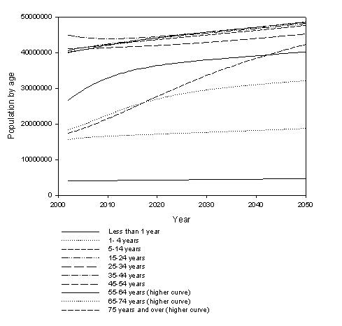
Figure 1. USA population projection 2002–2050: different age groups.
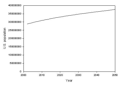
Figure 2. USA population projection 2002–2050.
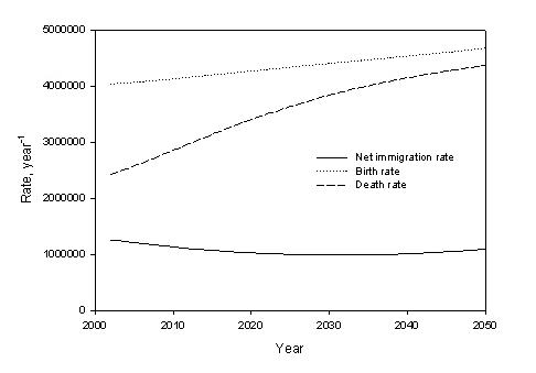
Figure 3. USA population projection 2002–2050: net immigration rate, birth rate, death rate.
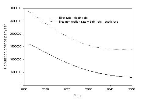
Figure 4. USA population projection 2002–2050: birth rate - death rate; net immigration rate + birth rate - death rate.
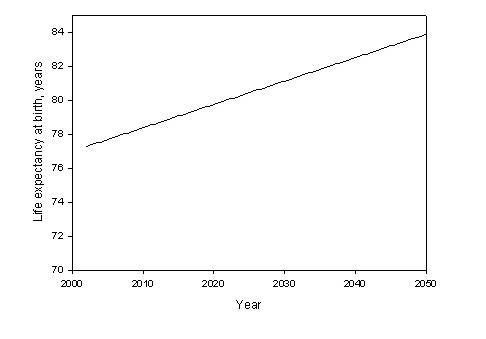
Figure 5. USA population projection 2002–2050: life expectancy at birth.
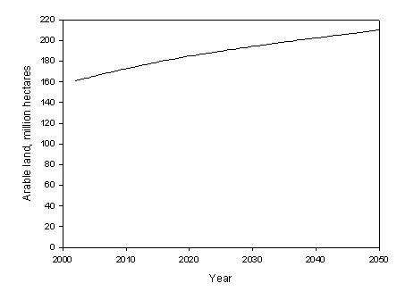
Figure 6. USA population projection 2002–2050: arable land for food production.
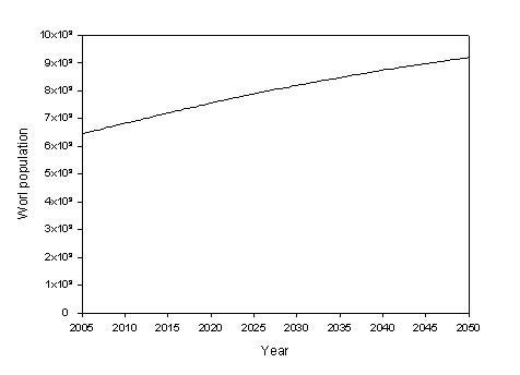
Figure 7. World population projection 2005–2050.
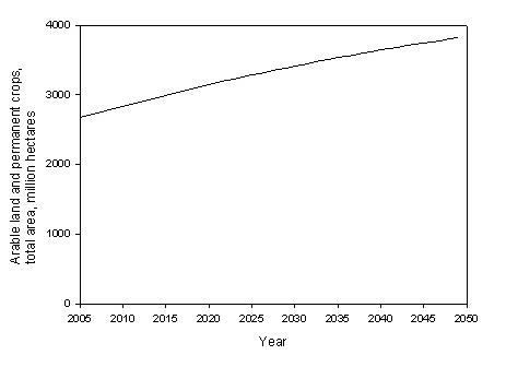
Figure 8. World population projection 2005–2050: arable land for food production.
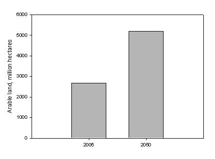
Figure 9. World arable land in 2005 and 2050 assuming that in 2050 20% of 111 million barrels per day of 2025 estimated petroleum production is replaced by wheat ethanol.
World population projection 2005–2050 – problem setup:
Differential equations| 1 | d(A)/d(t) = rate / 100 * A |
| World population |
Explicit equations
| 1 | rate = (-5.228E-07 * t ^ 4 + 5.2237E-05 * t ^ 3 - 1.6171E-03 * t ^ 2 - 1.1655E-03 * t + 1.1433) |
| Average annual growth rate of world population, % [US Census Bureau] | |
| 2 | INCREASE = A - 6451058790 |
| Population change compared to 2005 |
Matlab code
M-file WORLDpopulation.m:
function dYfuncvecdt = ODEfun(t,Yfuncvec);
A = Yfuncvec(1);
%Average annual growth rate of world population, % [US Census Bureau]
rate = (-5.228E-07 * t ^ 4 + 5.2237E-05 * t ^ 3 - 1.6171E-03 * t ^ 2 -
1.1655E-03 * t + 1.1433);
%Population change compared to 2005
INCREASE = A - 6451058790;
%World population
dAdt = rate / 100 * A;
dYfuncvecdt = [dAdt];
Command window:
>>
tspan = [0 45.]; % Range for the independent variable
>>
y0 = [6.451E+09]; % Initial values for the dependent variables
>> [t,y]=ode45('WORLDpopulation',tspan,y0);
>> plot(t,y(:,1));
>>
USA population projection 2002–2050 – problem setup:
Differential equations| 1 | d(A0_1)/d(t) = rbirth - rdeath0_1 - r0to1 + A0_1 / population0_45 * m |
| Population below 1 year | |
| 2 | d(A1_4)/d(t) = r0to1 - rdeath1_4 - r4to5 + A1_4 / population0_45 * m |
| Population at the age of 1-4 | |
| 3 | d(A5_14)/d(t) = r4to5 - rdeath5_14 - r14to15 + A5_14 / population0_45 * m |
| Population at the age of 5-14 | |
| 4 | d(A15_24)/d(t) = r14to15 - rdeath15_24 - r24to25 + A15_24 / population0_45 * m |
| Population at the age of 15-24 | |
| 5 | d(A25_34)/d(t) = r24to25 - rdeath25_34 - r34to35 + A25_34 / population0_45 * m |
| Population at the age of 25-34 | |
| 6 | d(A35_44)/d(t) = r34to35 - rdeath35_44 - r44to45 + A35_44 / population0_45 * m |
| Population at the age of 35-44 | |
| 7 | d(A45_54)/d(t) = r44to45 - rdeath45_54 - r54to55 |
| Population at the age of 45-44 | |
| 8 | d(A55_64)/d(t) = r54to55 - rdeath55_64 - r64to65 |
| Population at the age of 55-64 | |
| 9 | d(A65_74)/d(t) = r64to65 - rdeath65_74 - r74to75 |
| Population at the age of 65-74 | |
| 10 | d(A75_inf)/d(t) = r74to75 - rdeath75_inf |
| Population at the age of 75 and over | |
| 11 | d(B)/d(t) = rbirth |
| Birth rate | |
| 12 | d(D)/d(t) = rdeath0_1 + rdeath1_4 + rdeath5_14 + rdeath15_24 + rdeath25_34 + rdeath35_44 + rdeath45_54 + rdeath55_64 + rdeath65_74 + rdeath75_inf |
| Death rate |
Explicit equations
| 1 | population0_45 = A0_1 + A1_4 + A5_14 + A15_24 + A25_34 + A35_44 |
| Population below 45 in USA, immigration is allocated to this group | |
| 2 | Total_population = A0_1 + A1_4 + A5_14 + A15_24 + A25_34 + A35_44 + A45_54 + A55_64 + A65_74 + A75_inf |
| Total population of USA | |
| 3 | m = 320.759 * t ^ 2 - 18733.875 * t + 1257197.714 |
| Net immigration (second degree polynomial fitted to US Consensus Bureau prognosis 2002-2050) | |
| 4 | womanshare10_14 = 0.488 |
| Share of women at age group 10-14. In 2002, there was one woman at age group 10-14 who gave birth to her 4th child. | |
| 5 | birth_rate10_14 = 0.0007 * womanshare10_14 |
| Birth rate at age group 10-14 [National Vital Statistics Reports, Vol. 52, No. 10, December 17, 2003] | |
| 6 | womanshare15_44 = 0.495 |
| Share of women at age group 15-44. In 2002, there was one 15 year old woman who gave birth to her 6th child. | |
| 7 | birth_rate15_44 = 0.0648 * womanshare15_44 |
| Birth rate at age group 15-44 [National Vital Statistics Reports, Vol. 52, No. 10, December 17, 2003] | |
| 8 | womanshare45_50 = 0.5075 |
| Share of women at age group 45-50. | |
| 9 | birth_rate45_50 = 0.0005 * womanshare45_50 |
| Birth rate at age group 45-50-vuotiaat [National Vital Statistics Reports, Vol. 52, No. 10, December 17, 2003], In 2002, there were 263 women who had child (63 of them gave their first birth) | |
| 10 | rbirth = birth_rate10_14 * A5_14 / 2 + birth_rate15_44 * (A15_24 + A25_34 + A35_44) + birth_rate45_50 * A45_54 / 2 |
| Total birth rate | |
| 11 | Odo = 12.5 + 0.5 / 1.4 * 0.1375 * t |
| Life expectancy at 75, linear fit to US Census Bureau projection 2002-2050. 1.4-year life expectancy increase at birth corresponds to 0.5-year life expectancy increase at 75. | |
| 12 | r0to1 = 1 * A0_1 |
| Shift from the age group below 1 to the age group 1-4 | |
| 13 | r4to5 = 0.25 * A1_4 |
| Shift from the age group 1-4 to the age group 5-14 | |
| 14 | r14to15 = 0.1 * A5_14 |
| Shift from the age group 5-14 to the age group 15-24 | |
| 15 | r24to25 = 0.1 * A15_24 |
| Shift from the age group 15-24 to the age group 25-34 | |
| 16 | r34to35 = 0.1 * A25_34 |
| Shift from the age group 25-34 to the age group 35-44 | |
| 17 | r44to45 = 0.1 * A35_44 |
| Shift from the age group 35-44 to the age group 45-54 | |
| 18 | r54to55 = 0.1 * A45_54 |
| Shift from the age group 45-54 to the age group 55-64 | |
| 19 | r64to65 = 0.1 * A55_64 |
| Shift from the age group 55-64 to the age group 65-74 | |
| 20 | r74to75 = 0.1 * A65_74 |
| Shift from the age group 65-74 to the age group 75 and over | |
| 21 | rdeath0_1 = 0.00697 * A0_1 |
| Death rate at the age group below 1 | |
| 22 | rdeath1_4 = 0.00124 / 4 * A1_4 |
| Death rate at the age group 1-4 | |
| 23 | rdeath5_14 = 0.00174 / 10 * A5_14 |
| Death rate at the age group 5-14 | |
| 24 | rdeath15_24 = 0.00814 / 10 * A15_24 |
| Death rate at the age group 15-24 | |
| 25 | rdeath25_34 = 0.01029 / 10 * A25_34 |
| Death rate at the age group 25-34 | |
| 26 | rdeath35_44 = 0.02007 / 10 * A35_44 |
| Death rate at the age group 35-44 | |
| 27 | rdeath45_54 = 0.04315 / 10 * A45_54 |
| Death rate at the age group 45-54 | |
| 28 | rdeath55_64 = 0.09633 / 10 * A55_64 |
| Death rate at the age group 55-64 | |
| 29 | rdeath65_74 = 0.22111 / 10 * A65_74 |
| Death rate at the age group 65-74 | |
| 30 | d75_inf = 1 / Odo |
| Probability of death at the age group 75 and over (during one year) | |
| 31 | rdeath75_inf = d75_inf * A75_inf |
| Death rate at the age group 75 and over | |
| 32 | rdeath = rdeath0_1 + rdeath1_4 + rdeath5_14 + rdeath15_24 + rdeath25_34 + rdeath35_44 + rdeath45_54 + rdeath55_64 + rdeath65_74 + rdeath75_inf |
| Total death rate | |
| 33 | Life_expectancy_at_birth = 77.3 + 0.1375 * t |
| Life expectancy at birth, linear fit to US Census Bureau projection 2002-2050. |
Matlab code
M-file USApopulation.m:
function dYfuncvecdt = ODEfun(t,Yfuncvec);
A0_1 = Yfuncvec(1);
A1_4 = Yfuncvec(2);
A5_14 = Yfuncvec(3);
A15_24 = Yfuncvec(4);
A25_34 = Yfuncvec(5);
A35_44 = Yfuncvec(6);
A45_54 = Yfuncvec(7);
A55_64 = Yfuncvec(8);
A65_74 = Yfuncvec(9);
A75_inf = Yfuncvec(10);
B = Yfuncvec(11);
D = Yfuncvec(12);
%Population below 45 in USA, immigration is allocated to this group
population0_45 = A0_1 + A1_4 + A5_14 + A15_24 + A25_34 + A35_44;
%Total population of USA
Total_population = A0_1 + A1_4 + A5_14 + A15_24 + A25_34 + A35_44 + A45_54 +
A55_64 + A65_74 + A75_inf;
%Net immigration (second degree polynomial fitted to US Consensus Bureau
prognosis 2002-2050)
m = 320.759 * t ^ 2 - 18733.875 * t + 1257197.714;
%Share of women at age group 10-14. In 2002, there was one woman at age group
10-14 who gave birth to her 4th child.
womanshare10_14 = 0.488;
%Birth rate at age group 10-14 [National Vital Statistics Reports, Vol. 52, No.
10, December 17, 2003]
birth_rate10_14 = 0.0007 * womanshare10_14;
%Share of women at age group 15-44. In 2002, there was one 15 year old woman who
gave birth to her 6th child.
womanshare15_44 = 0.495;
%Birth rate at age group 15-44 [National Vital Statistics Reports, Vol. 52, No.
10, December 17, 2003]
birth_rate15_44 = 0.0648 * womanshare15_44;
%Share of women at age group 45-50.
womanshare45_50 = 0.5075;
%Birth rate at age group 45-50-vuotiaat [National Vital Statistics Reports, Vol.
52, No. 10, December 17, 2003],
In 2002, there were 263 women who had child
(63 of them gave their first birth)
birth_rate45_50 = 0.0005 * womanshare45_50;
%Total birth rate
rbirth = birth_rate10_14 * A5_14 / 2 + birth_rate15_44 * (A15_24 + A25_34 +
A35_44) + birth_rate45_50 * A45_54 / 2;
%Life expectancy at 75, linear fit to US Census Bureau projection 2002-2050.
1.4-year life expectancy increase at birth corresponds to 0.5-year life
expectancy increase at 75.
Odo = 12.5 + 0.5 / 1.4 * 0.1375 * t;
%Shift from the age group below 1 to the age group 1-4
r0to1 = 1 * A0_1;
%Shift from the age group 1-4 to the age group 5-14
r4to5 = 0.25 * A1_4;
%Shift from the age group 5-14 to the age group 15-24
r14to15 = 0.1 * A5_14;
%Shift from the age group 15-24 to the age group 25-34
r24to25 = 0.1 * A15_24;
%Shift from the age group 25-34 to the age group 35-44
r34to35 = 0.1 * A25_34;
%Shift from the age group 35-44 to the age group 45-54
r44to45 = 0.1 * A35_44;
%Shift from the age group 45-54 to the age group 55-64
r54to55 = 0.1 * A45_54;
%Shift from the age group 55-64 to the age group 65-74
r64to65 = 0.1 * A55_64;
%Shift from the age group 65-74 to the age group 75 and over
r74to75 = 0.1 * A65_74;
%Death rate at the age group below 1
rdeath0_1 = 0.00697 * A0_1;
%Death rate at the age group 1-4
rdeath1_4 = 0.00124 / 4 * A1_4;
%Death rate at the age group 5-14
rdeath5_14 = 0.00174 / 10 * A5_14;
%Death rate at the age group 15-24
rdeath15_24 = 0.00814 / 10 * A15_24;
%Death rate at the age group 25-34
rdeath25_34 = 0.01029 / 10 * A25_34;
%Death rate at the age group 35-44
rdeath35_44 = 0.02007 / 10 * A35_44;
%Death rate at the age group 45-54
rdeath45_54 = 0.04315 / 10 * A45_54;
%Death rate at the age group 55-64
rdeath55_64 = 0.09633 / 10 * A55_64;
%Death rate at the age group 65-74
rdeath65_74 = 0.22111 / 10 * A65_74;
%Probability of death at the age group 75 and over (during one year)
d75_inf = 1 / Odo;
%Death rate at the age group 75 and over
rdeath75_inf = d75_inf * A75_inf;
%Total death rate
rdeath = rdeath0_1 + rdeath1_4 + rdeath5_14 + rdeath15_24 + rdeath25_34 +
rdeath35_44 + rdeath45_54 + rdeath55_64 + rdeath65_74 + rdeath75_inf;
%Life expectancy at birth, linear fit to US Census Bureau projection 2002-2050.
Life_expectancy_at_birth = 77.3 + 0.1375 * t;
%Population below 1 year
dA0_1dt = rbirth - rdeath0_1 - r0to1 + A0_1 / population0_45 * m;
%Population at the age of 1-4
dA1_4dt = r0to1 - rdeath1_4 - r4to5 + A1_4 / population0_45 * m;
%Population at the age of 5-14
dA5_14dt = r4to5 - rdeath5_14 - r14to15 + A5_14 / population0_45 * m;
%Population at the age of 15-24
dA15_24dt = r14to15 - rdeath15_24 - r24to25 + A15_24 / population0_45 * m;
%Population at the age of 25-34
dA25_34dt = r24to25 - rdeath25_34 - r34to35 + A25_34 / population0_45 * m;
%Population at the age of 35-44
dA35_44dt = r34to35 - rdeath35_44 - r44to45 + A35_44 / population0_45 * m;
%Population at the age of 45-44
dA45_54dt = r44to45 - rdeath45_54 - r54to55;
%Population at the age of 55-64
dA55_64dt = r54to55 - rdeath55_64 - r64to65;
%Population at the age of 65-74
dA65_74dt = r64to65 - rdeath65_74 - r74to75;
%Population at the age of 75 and over
dA75_infdt = r74to75 - rdeath75_inf;
%Birth rate
dBdt = rbirth;
%Death rate
dDdt = rdeath0_1 + rdeath1_4 + rdeath5_14 + rdeath15_24 + rdeath25_34 +
rdeath35_44 + rdeath45_54 + rdeath55_64 + rdeath65_74 + rdeath75_inf;
dYfuncvecdt = [dA0_1dt; dA1_4dt; dA5_14dt; dA15_24dt; dA25_34dt; dA35_44dt;
dA45_54dt; dA55_64dt; dA65_74dt; dA75_infdt; dBdt; dDdt];
Command window:
>> tspan = [0 48.]; % Range for the independent variable
>> y0 = [4.034E+06; 1.558E+07; 4.104E+07; 4.059E+07; 3.993E+07; 4.492E+07; 4.008E+07; 2.66E+07; 1.827E+07; 1.733E+07; 0; 0]; % Initial values for the dependent variables
>> [t,y]=ode45('USApopulation',tspan,y0);
>> plot(t,y(:,1),t,y(:,2),t,y(:,3),t,y(:,4),t,y(:,5),t,y(:,6),t,y(:,7),t,y(:,8),t,y(:,9),t,y(:,10));
>>